3.2 R语言性能监控工具Rprof
问题
如何找到性能瓶颈?

引言
随着R语言使用越来越深入,R语言的计算性能问题越来越突显。如何能清楚地了解一个算法对CPU的耗时,将成为性能优化的关键因素。值得庆幸的是,R的基础库提供了性能监控的函数Rprof()。
3.2.1 Rprof()函数介绍
Rprof()函数是R语言核心包自带的一个性能数据日志函数,可以打印出函数的调用关系和CPU耗时的数据。然后通过summaryRprof()函数分析Rprof()生成的日志数据,获得性能报告。最后使用profr库的plot函数,对报告进行可视化。
3.2.2 Rprof()函数的定义
本节使用的系统环境是:
- Win7 64bit
- R: 3.0.1 x86_64-w64-mingw32/x64 b4bit
注:Rprof和profr同时支持Win7环境和Linux环境。
Rprof()函数在基础包utils中定义,不用安装,直接可以使用。
查看Rprof()函数的定义
~ R  # 启动R程序
> Rprof   # 查看Rprof()函数定义
function (filename = "Rprof.out", append = FALSE, interval = 0.02,
memory.profiling = FALSE, gc.profiling = FALSE, line.profiling = FALSE,
numfiles = 100L, bufsize = 10000L)
{
if (is.null(filename))
filename <- ""
invisible(.External(C_Rprof, filename, append, interval,
memory.profiling, gc.profiling, line.profiling, numfiles,
bufsize))
}
<bytecode: 0x000000000d8efda8>
Rprof()函数用来生成记录性能指标的日志文件,通常我们只需要指定输出文件(filename)就可以了。
3.2.3 Rprof()函数使用: 股票数据分析案例
以本书6.6节股票数据作为测试数据集,数据文件为000000_0.txt, 1.38 MB,在随书的代码文件中可以找到。本节只是性能测试,关于数据的业务含义,请参看6.6节内容。
> bidpx1<-read.csv(file="000000_0.txt",header=FALSE)
> names(bidpx1)<-c("tradedate","tradetime","securityid","bidpx1","bidsize1","offerpx1", "offersize1")
> bidpx1$securityid<-as.factor(bidpx1$securityid)
> head(bidpx1)
  tradedate tradetime securityid bidpx1 bidsize1 offerpx1 offersize1
1  20130724    145004     131810  2.620     6960    2.630      13000
2  20130724    145101     131810  2.860    13880    2.890       6270
3  20130724    145128     131810  2.850   327400    2.851       1500
4  20130724    145143     131810  2.603    44630    2.800      10650
5  20130724    144831     131810  2.890    11400    3.000      77990
6  20130724    145222     131810  2.600  1071370    2.601      35750


> object.size(bidpx1)
1299920 bytes
字段解释
- tradedate: 交易日期
- tradetime: 交易时间
- securityid: 股票ID
- bidpx1: 买一价
- bidsize1: 买一量
- offerpx1: 卖一价
- offersize1: 卖一量
计算任务:以securityid分组,计算每小时的买一价的平均值和买一量的总量。
> library(plyr)  # 加载plyr包,用于数据处理
> fun1<-function(){  # 数据处理封装到fun1()函数
+     datehour<-paste(bidpx1$tradedate,substr(bidpx1$tradetime,1,2),sep="")
+     df<-cbind(datehour,bidpx1[,3:5])
+     ddply(bidpx1,.(securityid,datehour),summarize,price=mean(bidpx1),size=sum(bidsize1))
+ }
> head(fun1())

  securityid   datehour    price      size
1     131810 2013072210 3.445549 189670150
2     131810 2013072211 3.437179 131948670
3     131810 2013072212 3.421000       920
4     131810 2013072213 3.509442 299554430
5     131810 2013072214 3.578667 195130420
6     131810 2013072215 1.833000    718940
以system.time()函数查看fun1()函数运行时间,运行2次,系统耗时近似,确定第二次没有缓存。
> system.time(fun1())
用户 系统 流逝
0.08 0.00 0.07
> system.time(fun1())
用户 系统 流逝
0.06 0.00 0.06
用Rprof()函数记录性能指标数据,并输出到文件。
> file<-"fun1_rprof.out"                       # 定义性能日志的输出文件位置
> Rprof(file)                                   # 开始性能监控
> fun1()                                         # 执行计算函数
> Rprof(NULL)                                   # 停止性能监控,并输出到文件
查看生成的性能指标文件:fun1_rprof.out。
~ vi fun1_rprof.out   # 用vi编辑器打开文件
sample.interval=20000
"substr" "paste" "fun1"
"paste" "fun1"
"structure" "splitter_d" "ddply" "fun1"
".fun" "" ".Call" "loop_apply" "llply" "ldply" "ddply" "fun1"
".fun" "" ".Call" "loop_apply" "llply" "ldply" "ddply" "fun1"
".fun" "" ".Call" "loop_apply" "llply" "ldply" "ddply" "fun1"
"[[" "rbind.fill" "list_to_dataframe" "ldply" "ddply" "fun1"
我们其实看不明白这个日志,不知道它到底有什么意义。所以,还要通过summaryRprof()函数来解析这个日志。
通过summaryRprof函数查看统计报告。
> summaryRprof(file)  # 读入文件
$by.self

 self.time self.pct total.time total.pct
".fun"           0.06    42.86       0.06     42.86
"paste"          0.02    14.29       0.04     28.57
"[["             0.02    14.29       0.02     14.29
"structure"      0.02    14.29       0.02     14.29
"substr"         0.02    14.29       0.02     14.29

$by.total

   total.time total.pct self.time self.pct
"fun1"                    0.14    100.00      0.00     0.00
"ddply"                   0.10     71.43      0.00     0.00
"ldply"                   0.08     57.14      0.00     0.00
".fun"                    0.06     42.86      0.06    42.86
".Call"                   0.06     42.86      0.00     0.00
""                        0.06     42.86      0.00     0.00
"llply"                   0.06     42.86      0.00     0.00
"loop_apply"              0.06     42.86      0.00     0.00
"paste"                   0.04     28.57      0.02    14.29
"[["                      0.02     14.29      0.02    14.29
"structure"               0.02     14.29      0.02    14.29
"substr"                  0.02     14.29      0.02    14.29
"list_to_dataframe"       0.02     14.29      0.00     0.00
"rbind.fill"              0.02     14.29      0.00     0.00
"splitter_d"              0.02     14.29      0.00     0.00

$sample.interval
[1] 0.02
$sampling.time
[1] 0.14
数据解释:
- $by.self是当前函数的耗时情况,其中self.time为实际运行时间,total.time为累计运行时间。
- $by.total是整体函数调用的耗时情况,其中self.time为实际运行时间,total.time为累计运行时间。
从$by.self观察,我们发现时间主要花在 .fun函数。
- fun: 实际运行时间0.06,占当前函数时间的42.86%。
- paste:实际运行时间0.02,占当前函数时间的14.29% 。
- "[[":实际运行时间0.02,占当前函数时间的13.29%。
- "structure":实际运行时间0.02,占当前函数时间的14.29%。
- "substr":实际运行时间0.02,占当前函数时间的14.29%。
对应在 $by.total中,从底到上(1-4),按执行顺序排序。
- 4 fun1: 累计运行时间0.14,占总累计运行时间的 100%,实际运行时间0.00。
- 3 .fun: 累计运行时间0.06,占总累计运行时间的 42.86 %,实际运行时间0.06。
- 2 paste:累计运行时间0.04,占总累计运行时间的 28.57%,实际运行时间0.02。
- 1 splitter_d:累计运行时间0.02,占总累计运行时间的 14.297%,实际运行时间0.00。
这样我们就知道了每个调用函数的CPU时间,进行性能优化就从最耗时的函数开始。
3.2.4 Rprof()函数使用: 数据下载案例
我们先安装 stockPortfolio包,需要通过stockPortfolio下载股票行情的数据,然后使用Rprof()函数监控下载过程的程序耗时情况。
> install.packages("stockPortfolio")  # 安装stockPortfolio包
> library(stockPortfolio)  # 加载stockPortfolio包
> fileName <- "Rprof2.log"
> Rprof(fileName)  # 开始性能监控
> gr <- getReturns(c("GOOG", "MSFT", "IBM"), freq="week")  # 下载Google,微软,IBM的股票数据
> gr

Time Scale: week
Average Return
   GOOG        MSFT         IBM
0.004871890 0.001270758 0.001851121

> Rprof(NULL)  # 完成性能监控
> summaryRprof(fileName)$by.total[1:8,]   # 查看性能报告

   total.time total.pct self.time self.pct
"getReturns"              6.76    100.00      0.00     0.00
"read.delim"              6.66     98.52      0.00     0.00
"read.table"              6.66     98.52      0.00     0.00
"scan"                    4.64     68.64      4.64    68.64
"file"                    2.02     29.88      2.02    29.88
"as.Date"                 0.08      1.18      0.02     0.30
"strptime"                0.06      0.89      0.06     0.89
"as.Date.character"       0.06      0.89      0.00     0.00

从打印出的的 $by.total 前8条最耗时的记录来看,实际运行时间(self.time) 主要花在file:2.02, scan:4.64
3.2.5 用profr包可视化性能指标
profr包提供了对Rprof()函数输出的性能报告可视化展示功能,比summaryRprof()的纯文字的报告,要更友好,有利于阅读。
首先,我们要安装profr包。
> install.packages("profr")  # 安装profr
> library(profr) # 加载profr包
> library(ggplot2)  # 用ggplot2包来画图, 加载ggplot2包
数据可视化:第一个例子,股票数据分析案例。
> file<-"fun1_rprof.out"> plot(parse_rprof(file))        # plot画图
> ggplot(parse_rprof(file))       # ggplot2画图
该代码段产生图3-1和图3-2。
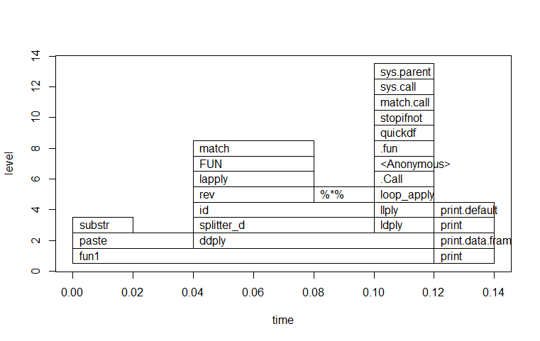
图3-1 第一个例子中用plot画的图
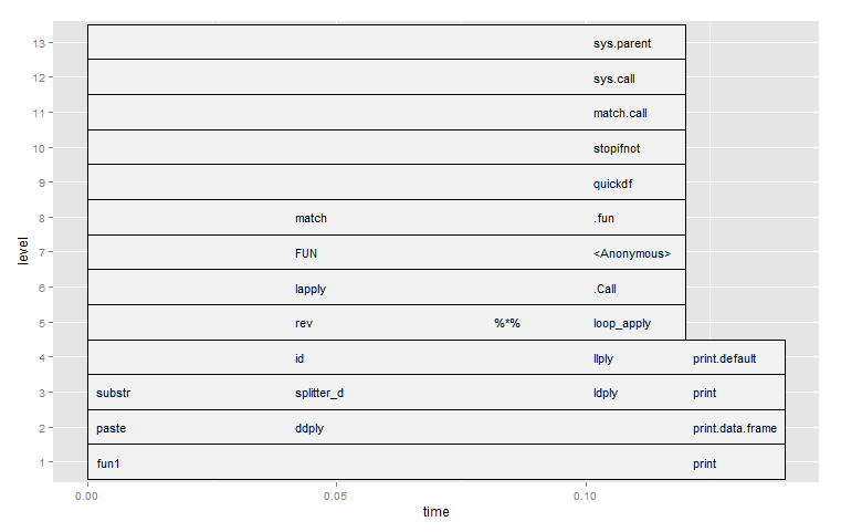
图3-2 第一个例子中用ggplot2画的图
数据可视化:第二个例子,数据下载案例。> fileName <- "Rprof2.log"
> plot(parse_rprof(fileName))
> ggplot(parse_rprof(fileName))
该代码段生成图3-3和图3-4。
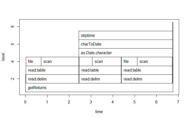
图3-3 第二个例子中用plot画的图
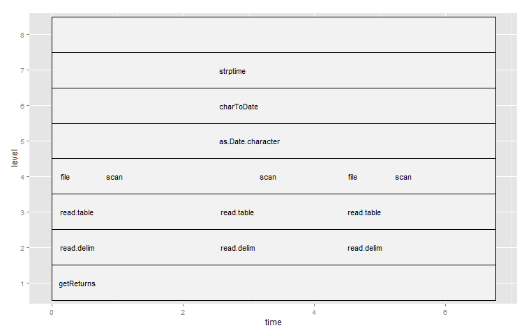
图3-4 第二个例子中用ggplot2画的图
3.2.6 Rprof的命令行使用
Rprof的命令行方法,用来方便地查看日志文件。
1 查看Rprof命令行帮助
~ D:\workspace\R\preforemence\Rprof>R CMD Rprof --help
Usage: R CMD Rprof [options] [file]

Post-process profiling information in file generated by Rprof().
Options:

 -h, --help       print short help message and exit
  -v, --version    print version info and exit
  --lines          print line information
  --total          print only by total
  --self           print only by self
  --linesonly      print only by line (implies --lines)
  --min%total=     minimum % to print for 'by total'
  --min%self=      minimum % to print for 'by self'
命令行解释
- -h, –help: 打印帮助信息。
- -v, –version: 打印版本信息。
- –lines: 打印显示多行。
- –total: 只显示总数。
- –self: 只显示私有的。
- –linesonly: 只显示单行(配合–lines使用)。
- –min%total=: 显示total的不低于X的百分比。
- –min%self=: 显示self的不低于X的百分比。
2 Rprof命令行使用
显示完整的报告。
~ D:\workspace\R\preforemence\Rprof>R CMD Rprof fun1_rprof.out
Each sample represents 0.02 seconds.
Total run time: 0.14 seconds.
Total seconds: time spent in function and callees.
Self seconds: time spent in function alone.

   %       total       %        self
 total    seconds     self    seconds    name
 100.0      0.14       0.0      0.00     "fun1"
  71.4      0.10       0.0      0.00     "ddply"
  57.1      0.08       0.0      0.00     "ldply"
  42.9      0.06      42.9      0.06     ".fun"
  42.9      0.06       0.0      0.00     ".Call"
  42.9      0.06       0.0      0.00     ""
  42.9      0.06       0.0      0.00     "llply"
  42.9      0.06       0.0      0.00     "loop_apply"
  28.6      0.04      14.3      0.02     "paste"
  14.3      0.02      14.3      0.02     "[["
  14.3      0.02      14.3      0.02     "structure"
  14.3      0.02      14.3      0.02     "substr"
  14.3      0.02       0.0      0.00     "list_to_dataframe"
  14.3      0.02       0.0      0.00     "rbind.fill"
  14.3      0.02       0.0      0.00     "splitter_d"

 %        self       %      total
  self    seconds    total   seconds    name
  42.9      0.06      42.9      0.06     ".fun"
  14.3      0.02      28.6      0.04     "paste"
  14.3      0.02      14.3      0.02     "[["
  14.3      0.02      14.3      0.02     "structure"
  14.3      0.02      14.3      0.02     "substr"
只显示total指标,占用时间不低于50%的部分。
~ D:\workspace\R\preforemence\Rprof>R CMD Rprof --total --min%total=50 fun1_rprof.out
Each sample represents 0.02 seconds.
Total run time: 0.14 seconds.
Total seconds: time spent in function and callees.
Self seconds: time spent in function alone.

  %       total       %        self
 total    seconds     self    seconds    name
 100.0      0.14       0.0      0.00     "fun1"
  71.4      0.10       0.0      0.00     "ddply"
  57.1      0.08       0.0      0.00     "ldply"
我们可以通过Rprof进行性能调优,提高代码的性能,让R语言的计算不再是瓶颈。